
Transformers in Computer Vision
This blog post highlights the ongoing collaboration between Anyline and Machine Learning researchers from the LIT AI Lab at Johannes Kepler University Linz.
In the last few years, the concept of Transformers has completely revolutionized machine learning, and has achieved state-of-the-art performance in various tasks and domains. Since their introduction in 2017 [1], Transformers have replaced recurrent neural networks (RNNs) in many natural language processing (NLP) problems such as sequence classification, extractive question answering, language modeling, and others.
However, recent research demonstrates that Transformers outperform convolutional neural networks, and can successfully solve various Computer Visions tasks, including segmentation and even optical character recognition (OCR).
This blog post presents critical concepts and notions related to Transformer neural networks. In addition, it provides an overview of the state-of-the-art research focusing on transformer applications in Computer Vision and, in particular, OCR.
How does a Transformer work?
The original Transformer architecture [1] consists of two blocks: an encoder and a decoder. However, modern applications often use only one of these blocks, depending on the task. To put it simply, one can say that the encoder part is responsible for analyzing how pieces of the input information relate to each other. The decoder part is responsible for predicting the next token in a sequence based on the contextual information from the encoder. Language modeling often uses only the decoder block (for example, GPT-3 [2]), whereas for example, Named Entity Recognition or Part-of-Speech tagging uses only the encoder part (BERT, for instance [3]).
Since this blog is about Transformers for computer vision, we will focus on the encoder part as it’s utilized in most of the vision transformer applications. Then we briefly introduce the decoder part.
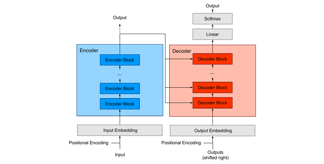
Figure 1 – Generalized schematic of the Transformer
The input to a Transformer network is typically sequential data transformed by a learnable embedding matrix. The latter is usually summed up with the so-called positional encoding to preserve the positional relationship information between individual tokens within the sequence. The number N of token embeddings used at one step is fixed, so we only use parts of a sequence if the whole sequence is too long. These embeddings are then fed into the Transformer Encoder, which consists of multiple layers of Encoder Blocks. The output of the last Encoder Block is also the output of the entire Encoder. Depending on the application, this output can be further processed using a Transformer Decoder, a Feed-Forward Network, or a Linear Layer with a Softmax Layer.

Figure 2 – Schematics of the Encoder Block
The Encoder Block (Figure 2) consists of a Self-Attention Layer and a Feed-Forward Network. The self-attention layer emphasizes the essential parts of the input data and suppresses the rest. The self-attention (also intra-attention) indicates how related a particular token is to all other tokens in the matrix X ∈ℝ(N⨯d_model), where d_model is the dimension of embedding which is used as input and output of the encoder block, N denotes the number of tokens. In NLP, for instance, this mechanism could pinpoint the noun that a pro-form represents.
Generally speaking, the attention is calculated based on three inputs: The Query (Q), the Key (K) and the Value (V). For a basic self-attention Q, K and V are obtained by multiplying X with weights W_q, W_k∈ℝ(d_model⨯d_k), and W_v ∈ℝ(d_model⨯d_v), respectively. Here d_k, d_v are intrinsic dimensions of self-attention. The values of these matrices are learned during the training.

When using multiple heads, we use different linear transformations W_i,q, W_i,k, and W_i,v – one for each of the h heads (i = 1,2,…,h). At the end, the resulting Attention Matrices, i.e. the outputs of the Attention for each head, are concatenated into a matrix Z∈ℝ(N⨯h d_v) and multiplied with the weight matrix WO∈ℝ(h d_v⨯d_model), which is jointly trained with the model. In case of h heads d_v is chosen d_v = d_model / h. The multiple heads allow the neural network to learn various relations of the tokens and can therefore capture different contextual information. Figure 3 shows the complete self-attention mechanism.
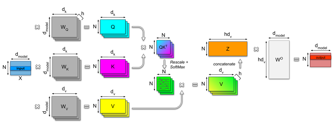
Figure 3 – Schematics of the self-attention mechanism
For training, some tokens of the input matrix X can be masked out. This masking mechanism ensures that the network attends only to the specific tokens in the sequence while ignoring the others. For example, the decoder part of the Transformer uses the masking mechanism to guarantee that the network’s output for a given token attends only to the previous tokens in the sequence, and does not relate to the information from the future tokens. The Feed-Forward Network at the top of the Encoder Block usually consists of two Linear Layers with a ReLU activation function. Such a Feed-Forward Network typically has a higher intermediate dimension.

The normalization layers and residual connections are standard techniques for faster and more accurate training. To sum up, the Encoder part of the Transformer neural network comprises several Encoder Blocks stacked on top of each other. The output of the Encoder can then be used as input for the Decoder block as in the original paper [1]. Alternatively, it can be processed directly as we can see for the Transformers in Computer Vision.
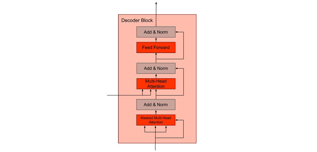
Figure 4 – Schematics of the Decoder Block
Decoders (Figure 4) have a Masked Multi-Head Attention as the first layer. It masks all consecutive tokens of the input to the decoder – for this layer the input is the output of the network of the last token. This ensures that the decoder learns to predict which token will follow after a particular sequence. In the next layer, the decoder is connected to the encoder by taking the output of the decoder as Q and K to its multi-head attention. Thus, the decoder learns to predict the next token in the sequence.
How are Transformers used in Computer Vision?
After the Transformer’s success in NLP tasks, it was only a matter of time before it would be applied to images. The first, and most obvious question that then arose was: what are the tokens in this case, and how do we feed an image to the transformer? As it turns out, using each pixel as a token would lead to a hefty computational load. Let us, for example, take an image of 256 x 256 in grayscale. This results in 65 536 pixels, and now we have to calculate how much each of them attends to all the other pixels. To calculate this, we will need to perform 655362 = 4 294 967 296 calculations, which is very slow to evaluate on today’s hardware, and it would be quadratically more difficult working with higher resolution images. For this reason, the famous Image GPT [4] works with low resolutions of 32×32, 48×48, and 64×64 due to computational costs. In the following example, we will proceed with the same approach and rescale our example image to 64×64 image for the sake of simplicity of the following computations (Figure 5).
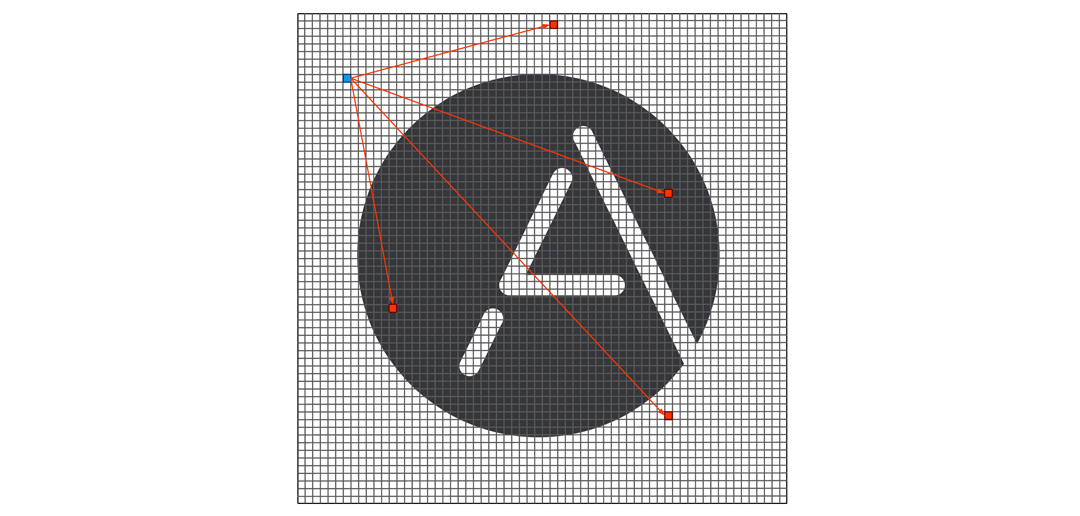
Figure 5 – Example of pixel-wise attention computation. In blue – pixel for which attention is computed, in red – pixels which are used in this process (in reality all pixels will be used, we use limited number of pixels for demonstration purpose)
While it was not yet clear how to use transformers on images, the first attempts to utilize the attention mechanism with CNNs were done in papers [5, 6]. Such approaches apply the attention mechanism to the feature maps obtained from convolutional neural networks.
Let’s return to our example and propagate a sample image of 64×64 pixels through the CNN backbone. We assume that the output of the convolutional backbone is a feature map of the dimensions 4x4xN (Figure 6). Following the method proposed in [5], we will utilize attention mechanisms from Transformer neural networks and generate a dense attention map for every 1x1xN feature (Figure 6a, blue). We calculate the latter (Figure 6a, green) by attending the feature at the current position to the entire feature block. The final value at the particular position (Figure 6a, red) is obtained by multiplying the respective attention map with the original feature block of 4x4xN and aggregating over all the feature positions. We repeat the same procedure for all the positions to compute the resulting feature map. Since the above-described operation resembles non-local mean computation within the block, this method was named non-local. The criss-cross attention block (Figure 6b) improved the approach above. While keeping the same attention mechanism, the authors of [6] suggested computing weights only involving the features aligned horizontally and vertically with the feature at the current position (Figure 6b, blue). The same procedure is repeated twice. According to authors [6], this operation produces more discriminative features and also reduces the computation complexity from O(N^2) to O(N√N), where N is the number of input features. However, for every feature, this computation still has to be performed twice.
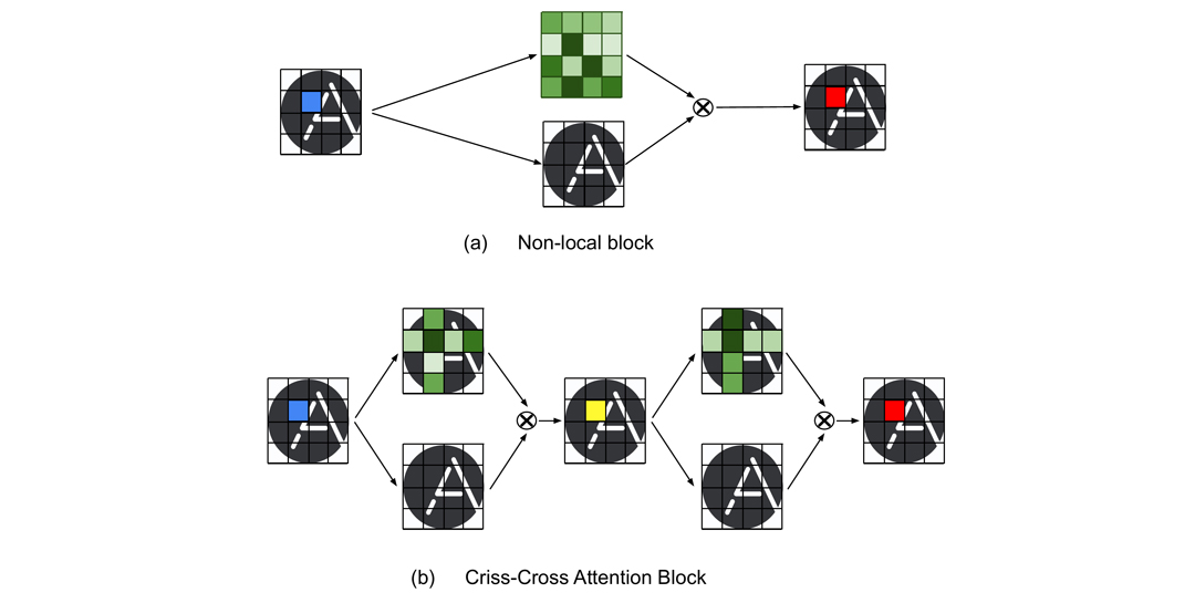
Figure 6 – Visual example of (a) Non-local and (b) Criss-Cross Attention blocks. In blue – pixel for which attention is computed, in red – resulting pixel with attention, in green – attention weights, in yellow – intermediate step.
The first image classification network purely based on transformers, known as a Vision Transformer (ViT), was introduced in the paper “An Image is Worth 16 x 16 Words: Transformers for Image Recognition at Scale” [7]. This approach deals with only the encoder part of the original transformers and splits images into non-overlapping patches, which are then interpreted as single tokens.These tokens are flattened and mapped to a fixed-length linear embedded space, which serves as standard input to the encoder part of the transformer (see Figure 7).
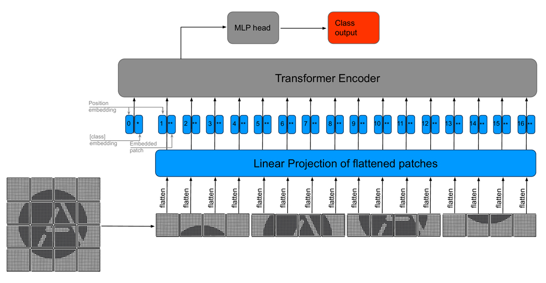
Figure 7 – Visual example of ViT for 64×64 image
Later stages calculate how much each patch attends to another patch. While the attention operation is still quadratic, the number of tokens decreases dramatically in this way. In our example, we would have 16 x 16 patches for a 64 x 64 image, which would result in 642 = 4096 calculations in the self-attention part of the Transformer. While ViT can compete with state-of-the-art CNN models, one of its main drawbacks is the fixed size of tokens and corresponding feature dimensions that cannot capture details at different dimensions.
In the paper “Swin Transformer: Hierarchical Vision Transformer using Shifted Vision” [8] the authors build a Transformer architecture that has linear computational complexity with respect to image size. The main idea is that instead of looking at the attention between all image patches, we further divide the image into windows. Then, the attention is calculated between the patches in the respective window, rather than between all the patches in the image.
The general architecture of the Shifted window (Swin) Transformer consists of several stages. We will have a closer look at Swin-T which has four stages (see, Figure 8). Each stage consists of a linear embedding or patch merging layer and two transformer units which are together denoted as a Swin Transformer Block – one consists of window multihead self-attention and the other one uses shifted window multihead self-attention.
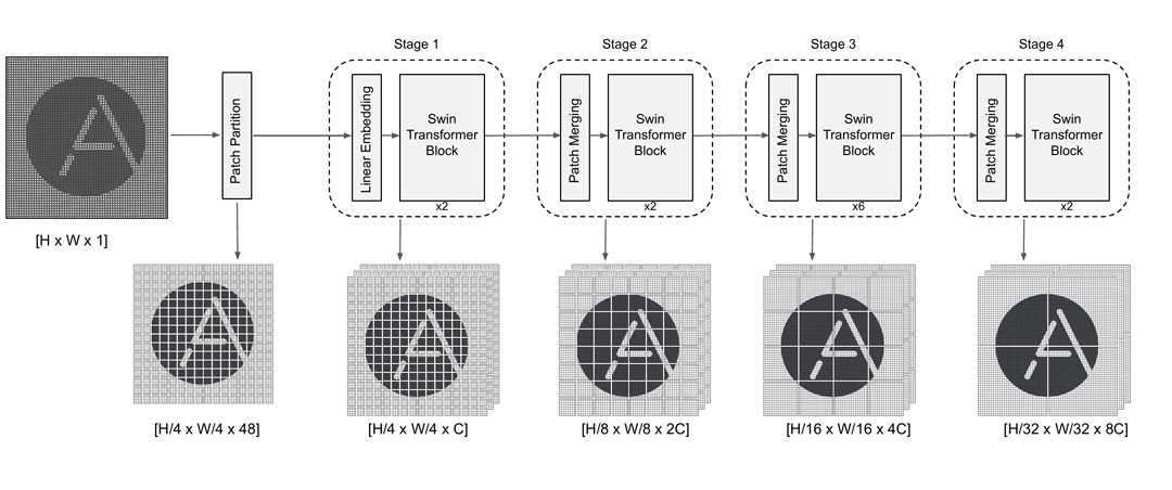
Figure 8 – visual example of Swin-T architecture and corresponding hierarchical representation of the input image
Let us go through the process and propagate a 64 x 64 image through the network.
- First, the image gets partitioned into patches in the same way as in the ViT described above. The only difference here is that the patches are of the size 4 x 4 instead of 16 x 16 with a dimension of 48 (4 x 4 x 3 for RGB images). In our example we will get 64 / 4 * 64 / 4 = 256 patches.
- Stage 1 consists of a linear embedding that projects the dimension of 48 of each patch into a C dimensional token. For a choice of C, please refer to the original paper. These tokens are fed into two Swin Transformer Blocks (see, Figure 8). We will have a closer look at Swin Transformer Block later.
- At stages 2-4, we have a patch merging mechanism, which concatenates patches obtained from the previous stage, followed by two Swin Transformer Blocks. Remember that for our example of 64 x 64 image at the stage 1 we had 64 / 4 * 64 / 4 = 256 patches. As for the stage 2 we will have 64 / 8 * 64 / 8 = 64 patches.
- Stage 3 and 4 repeat the same arrangement of operations as stage 2 (see, Figure 8). However, the number of Swin Transformer Blocks is changed to 6 and 2, respectively. As for our example this will result in 64 / 16 * 64 / 16 = 16 and 64 / 32 * 64 / 32 = 4 patches.
- It is important to mention that the matching mechanism does not change the size of the image itself, but changes an area where the attention is computed. (see, Figure 8)
Let’s have a look now at the Swin Transformer Block. The first part is the standard multi-head self-attention mechanism inside the windows. This makes the attention mechanism somewhat local again, which is compensated by the second part of the block – the shifted-window multihead self-attention. We denote the number of patches a window contains, by M x M.
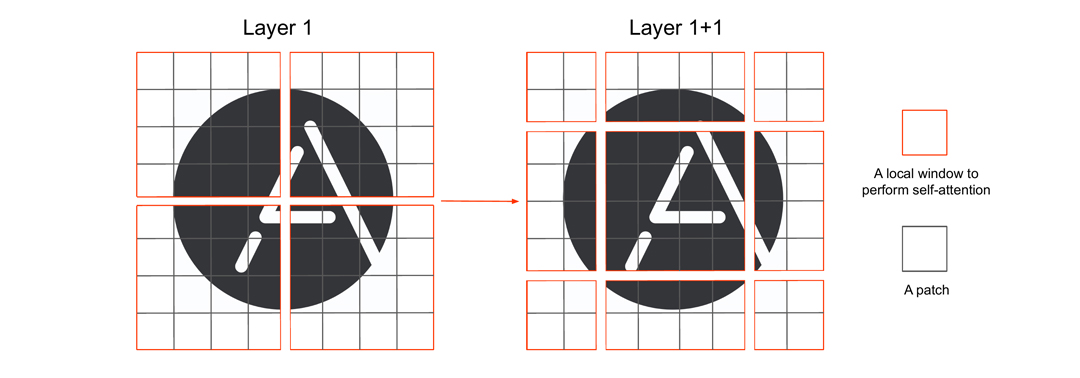
Figure 9 – Example of shifted self-attention for Stage 4 of Swin-T Transformer
The second part of the Swin Transformer Block displaces the windows by shifting the windows by two patches (generally M / 2) in the horizontal and vertical direction. It again performs self-attention on the resulting window configuration (see Figure 9). The shifted window self-attention solves the problem of not having connections across windows in comparison to the first part of the Swin Transformer Block. If we repeat the same procedure one more time, we will receive the so-called Two Successive Transformer Blocks, shown in Figure 10.
Given an image with h x w patches we can calculate that a regular multi-head self-attention module has a computational complexity of 4*h*w*C^2 + 2*(h*w)^2*C. In contrast, a window multi-head self-attention module has the complexity of 4*h*w*C^2 + 2*M^2*h*w*C. This shows that the complexity of the regular module is quadratic with respect to hw, while the window-based module is linear, because M is fixed!

Figure 10 [8] – Schematics of Two Successive Transformer Blocks
While Swin Transformers resolve computational complexity problems, preserved in ViT, these algorithms, unfortunately, share the identical drawback – they are extremely data-hungry. The authors claim that the ImageNet dataset with 1.3M images and 1k classes, relatively big for standard computer vision tasks, is too small for transformers. Their suggestion is to pre-train transformers with the JFT dataset, which contains 303M images and 18k classes, and distill this knowledge for further tasks. Yet, not everyone has sufficient resources to train on large datasets and the JFT dataset is not publicly available. As a solution to this, two approaches arise: Bidirectional Encoder Representations from Transformers (BERT) [3] and Bidirectional Encoder representation from Image Transformers (BEIT) [9]. The primary purpose of BERT is to provide pre-trained deep bidirectional language representation for different tasks such as question answering, translation, etc. BEIT was inspired by BERT as a pre-trained vision Transformers mainly for the classification and segmentation tasks. Such an approach utilizes a masked image model to predict the values of discrete visual tokens. The latter are produced by a VAE that is trained separately. The authors claim that with self-supervised pre-training on ImageNet-1k the BEIT outperforms V_iT for classification on ImageNet (79.9% ViT384-JFT300M vs 86.3% BEIT384-L). Although BEIT shows promising results, the recent research [10] indicates that masked auto-encoders (MAE) can enable pre-training of even larger models (ViT-H) on just ImageNet-1k and does not require an image tokenizer like BEIT. The authors of [10] demonstrate that their method has reasonable performance and generalizes well on downstream tasks: for ImageNet-1k, ViT-L (BEIT) has accuracy 85.2% vs. ViT-L (MAE) – 85.9%; however, ViT-H (MAE) – 87.8%.
Transformer applications in OCR
As you can see, Transformers are powerful tools that can be used in many deep learning applications. So, if they work so well both in text translation and image recognition, can they also be used in Optical Character Recognition (OCR)? The answer to this question was given by the recently published paper “TrOCR: Transformer-based Optical Character Recognition with Pre-trained Models” [11]. If you are unfamiliar with OCR, feel free to look at our blog-post What is OCR? Introduction to Optical Character Recognition, where we show what it is and how it works.
In short, TrOCR is an end-to-end pre-trained combination of image Transformer in the encoder part and text Transformer in the decoder part (see, Figure 11).
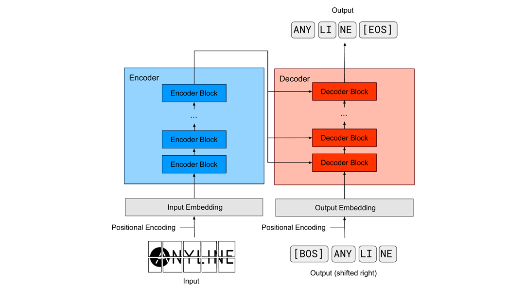
Figure 11 – Visual example of the TrOCR architecture
If we take a closer look, we will see that TrOCR utilizes a part from ViT – an original vanilla Transformer. As in ViT, the image is divided into fixed patches of size PxP, yet with no restriction to the size of P. After that, the images are flattened into 1D tokens and mapped to linear embedding space. In addition, the “[CLS]” token is added. At the encoder output this token will correspond to a representation of the entire input.. After this, a number of standard Transformer blocks can be used.
The decoder block receives features from the encoder block in the same manner as the original Transformer. The masking self-attention block in this case plays the same role as in the vanilla Transformer – it is required such that the Transformer would not cheat and see the ground truth while still performing prediction. TrOCR shows promising results for both handwritten and printed text. However, it still preserves the general problem of Transformers – a need for an enormous amount of data for pre-training.
To sum up, despite some disadvantages, Transformer neural networks is a very active and promising research area. Unlike recurrent neural networks, they can be pre-trained and fine-tuned for various domains, which makes them generalizable to many real-world applications. This blog demonstrates how Transformers can be used on images and how they can be applied in optical character recognition. But there are also many other applications of Transformers to be explored.
We strongly believe that innovation always goes together with our customers’ product quality and happiness. Therefore, stay tuned to see more! 🙂
References
- Vaswani, A., Shazeer, N., Parmar, N., Uszkoreit, J., Jones, L., Gomez, A. N., … & Polosukhin, I. (2017). Attention is all you need. In Advances in neural information processing systems (pp. 5998-6008).
- Brown, T. B., Mann, B., Ryder, N., Subbiah, M., Kaplan, J., Dhariwal, P., … & Amodei, D. (2020). Language models are few-shot learners. arXiv preprint arXiv:2005.14165.
- Devlin, J., Chang, M. W., Lee, K., & Toutanova, K. (2018). Bert: Pre-training of deep bidirectional transformers for language understanding. arXiv preprint arXiv:1810.04805.
- Chen, M., Radford, A., Child, R., Wu, J., Jun, H., Luan, D., & Sutskever, I. (2020, November). Generative pretraining from pixels. In International Conference on Machine Learning (pp. 1691-1703). PMLR.
- Wang, X., Girshick, R., Gupta, A., & He, K. (2018). Non-local neural networks. In Proceedings of the IEEE conference on computer vision and pattern recognition (pp. 7794-7803).
- Huang, Z., Wang, X., Huang, L., Huang, C., Wei, Y., & Liu, W. (2019). CCNet: Criss-cross attention for semantic segmentation. In Proceedings of the IEEE/CVF International Conference on Computer Vision (pp. 603-612).
- Dosovitskiy, A., Beyer, L., Kolesnikov, A., Weissenborn, D., Zhai, X., Unterthiner, T., … & Houlsby, N. (2020). An image is worth 16×16 words: Transformers for image recognition at scale. arXiv preprint arXiv:2010.11929.
- Liu, Z., Lin, Y., Cao, Y., Hu, H., Wei, Y., Zhang, Z., … & Guo, B. (2021). Swin transformer: Hierarchical vision transformer using shifted windows. arXiv preprint arXiv:2103.14030.
- Bao, H., Dong, L., & Wei, F. (2021). BEiT: BERT Pre-Training of Image Transformers. arXiv preprint arXiv:2106.08254.
- He, K., Chen, X., Xie, S., Li, Y., Dollár, P., Girshick., R. (2021). Masked Autoencoders are Scalable Vision Learners. arXiv preprint arXiv:2111.06377.
- Li, M., Lv, T., Cui, L., Lu, Y., Florencio, D., Zhang, C., … & Wei, F. (2021). TrOCR: Transformer-based Optical Character Recognition with Pre-trained Models. arXiv preprint arXiv:2109.10282.
Authors
Natalia Shepeleva (a), Dmytro Kotsur (a), Stefan Fiel (a), Sebastian Sanokowski (b), Sebastian Lehner (b)
(a) Anyline GmbH, (b) Institute for Machine Learning & LIT AI Lab, Johannes Kepler University Linz. The LIT AI Lab is supported by Land OÖ.


