Gradient Descent for Deep Learning & Motion Estimation
Discover how the mathematical tool of Gradient Descent is a shared technique in Deep Learning as well as in Motion Estimation.
We found something really striking in deep learning, which shares the same approach/technique as motion estimation, a completely different field. The purpose of motion estimation is to find the amount of motion in a video sequence. With deep learning, you can solve complex problems such as autonomous driving, recognition of handwritings or letters, and object detection. To our surprise, both of these fields, while having completely different goals, come close thanks to a mathematical tool called “Gradient Descent”.
Deep Learning from a Mathematical Perspective
Please don’t get scared by this title, there are going to be just a few simple formulas and a lot of text. Many problems in computer vision are solved using convolutional neural networks. When you want to build such a network, you put together different types of layers (convolutional, Relu, pooling, etc.) in a structure called a “model”. After this, the real magic starts: the model learns. And this happens as follows:
In order to understand if the model correctly learns the problem of interest, you need an accuracy measure. In other words, a mathematical formula that defines the delta between the predictions of the model and real examples (this set of examples is called “test set”). This mathematical formula is called “the cost function” and is usually composed of hundreds of parameters. Ideally, you’d like the distance between the model predictions and real data to be zero. However, this is often not possible (we live in an imperfect world), and you, therefore, calculate the parameters that give the best result when used in the function = the minimal distance. In the following formula there is an example of cost function:

where x is the input images, l(x) are the expected results, and y(x) is the neural network output.
In order to minimize the cost function, you use an algorithm (or one of its variations) called “Gradient Descent”. This algorithm solves non-linear systems of equations. Normally you can calculate the solution of a problem directly if it is expressed as a linear system. A linear system is a set of linear equations that have a solution. Everyone loves linear systems because they are easy and fast to solve. An example of a linear system follows:

Sadly, it is not always possible to describe problems with linear systems, especially for really interesting problems. In the case of a non-linear system, help comes from my friend introduced at the beginning of the article, the gradient descent.
I am sure that the non-linear problem has a solution, however, I cannot calculate it directly. Following the opposite direction of the gradient, the result will end up in a minimum of the cost function (this is mathematically proven but I will spare complicated details).
This process also works when the non-linear function is large, with hundreds of parameters, like in the case of deep learning functions.
Motion Estimation & Mathematicians’ Shortcut
You may wonder how this is connected with motion estimation. In order to calculate the motion available in a video, mathematicians describe the problem with a functional (a function of functions). Minimizing a functional is quite a challenge, so you take a shortcut: you minimize a function that has the same solution as the functional. Could you guess what type of function this is? Well done, if you guessed that this is a non-linear equation!
Let’s look at the assumptions for motion estimation:
The functional for motion estimation is based on a simple assumption: all the points belonging to an object preserve their color while the object moves. If my face (the object being looked at) moves 10 cm to the right, all the colors of my face remain exactly the same. The best possible movement from a mathematical point of view is the one that preserves all the colors. In mathematical terms:

where I is the input image, x and y are the coordinates of a point in the image, and u,v is the movement in x and y direction.
Since movement happens in microseconds, it is supposed to be smooth in space and time. In other words, from one frame to the next, the movement is small and coherent with the movement of the neighboring points. For example, if I move my face, as described above, all the points belonging to my face move with the same speed in the same direction. (You would not recognize my face if they were behaving differently).
In mathematical terms:

where ∇u and ∇v are respectively the gradients of the functions u and v. Like before u,v is the movement.
The result of all these assumptions put together is a function. Following further mathematical steps, this ends up in a non-linear equation to be minimized. And here comes again our good old friend, the gradient descent.
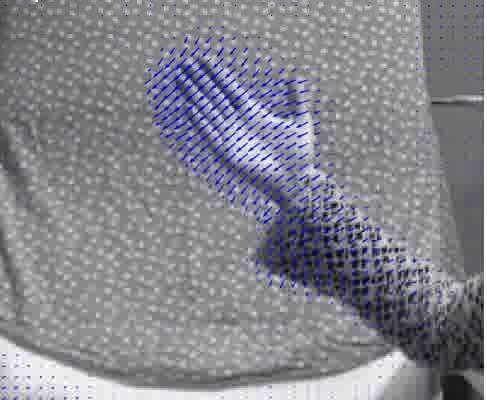
Let’s take a closer look at an example of motion estimation result:
In the following image, we see the arm of a person that is moving. The calculated motion is visualized with blue vectors. The direction and the size of each vector are proportional to the direction and size of the motion.

The “descent” in the “Gradient Descent” refers to the fact that one goes in the decreasing direction of the function, meaning that the function is minimized. You’re never alone with a Gradient Decent.


