Introduction to Graph Theory – Part 2

This post is a continuation of part 1 of our introduction to graph theory. In this part, I will explain the concept of dual graphs, region adjacency graphs, graph pyramids, and combinatorial pyramids. Even though these concepts may sound a bit difficult, the ideas behind them are relatively straight-forward. All of these constructs build on top of each other. Similarly, as in the previous part, where I explained why we needed to add weights and directions to the edges of a graph and attributes to the vertices, I will do my best to explain, why scientists needed to go further and further with these graph-related concepts. And since we are a Computer Vision company, I will do this all in the context of images 🙂

Image Graph

In the previous part, we introduced image graphs, which are specially used for storing and representing images. An image is essentially a set of grayscale or color values (pixel values) laid over a grid-like structure (pixel grid) and with a specific notion of neighborhood (4-, 6-, 8- neighborhood, etc.).  In a 4-neighborhood we say, that the left, right, top, and bottom pixels of a center pixel are its neighbors. In an 8-neighborhood, we additionally add the diagonal pixels as neighbors. When we represent an image using a graph, we store all of this information in the vertices (pixels), vertex attributes (pixel values), and edges (neighborhood relationships). We additionally can store the grayscale or color difference between neighboring pixels as the weights of the edges. One nice property of 4- and 6-connected image graphs is, that they are planar graphs. 8-connected image graphs are planar only up to a size of 3×3.

Figure 1: The construction of a 4-connected planar image graph.

Dual Graphs

Before we get to graph pyramids, I need to shortly explain the concept of dual graphs. One important property of planar graphs is, that they always have a dual graph. In the context of an image, the 4-connected image graph is then the primal graph. The vertices of the primal graph represent individual pixels, and the edges of the neighborhood relationships. In the dual graph, each vertex represents a face in the image graph. A face is essentially a 2×2 image patch. If you look at Figure 1, then one such face would be for example the 3 bottom left red pixels and 1 black pixel. Also, take a look at the figure below. Here the blue graph would be a primal graph. None of the blue edges are crossing each other, so it is a planar graph. We know, that each planar graph has a dual graph, so we can draw it in red color. Here, each red dual vertex represents a face, which is bounded by the edges of the blue primal graph. I know, so far this might be a little bit abstract, but don’t worry, in the next few paragraphs we will see, why we need the dual graph.

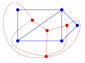
Figure 2: The blue graph is the primal graph, and the red graph is its dual graph.

Region Adjacency Graphs

Region adjacency graphs are simple graphs (no parallel edges, no self-loops), which represent the neighboring relationships of whole regions. A region is a collection of connected pixels, which share some properties. To make it simple, let’s say, that these properties are the color of the pixels. In the figure below, you can see a 4×6 pixels large image, where 7 neighboring pixels are red, 9 are black, and 8 are blue. When we combine these into regions, then we will have 3 regions, each of the three colors.

Figure 3: Pixels combined into whole regions.

And in the same way, an image graph with 24 vertices can be combined into a region adjacency graph with 3 vertices. This is shown in the figure below.

Figure 4: A region adjacency graph of the original 4×6 pixels large image.

This region adjacency graph effectively encodes the image into a different representation, which can store the layout of the image. It can describe, which regions are next to each other and which aren’t. Region adjacency graphs are however simple graphs, which is a disadvantage if you want to encode more complex configurations of regions. Imagine however a region being included in another region, or when a region is next to another region and they touch at multiple borders. How can you encode this setting with a region adjacency graph? Well, you can’t. Look at the figure below.

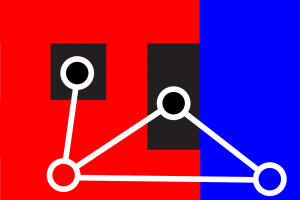
Figure 5: A more complex set of regions. The red region encloses one black region and has multiple borders with the blue region.

To be able to encode the setting in Figure 5, we would need a self-loop around the black enclosed region, and parallel edges between the red and blue region. With a simple region adjacency graph, this is however not possible. You could use an “extended” version of the region adjacency graph, which would be a multi-graph, but let’s look at a different approach, where we start with an image graph with 24 vertices, and use graph reduction operations, to end up with a dual graph, which encodes enclosed regions and multiple borders.

Graph Pyramid and Graph Reduction Operations

A graph pyramid is just a collection of multiple graphs, where the original image graph is at the bottom of the pyramid, and each level of the pyramid above holds a slightly smaller graph. These smaller graphs are produced by applying graph reduction operations to the graph in the level below. These reduction operations can be bound to vertices, or to edges, but essentially they are equivalent. We can for example merge two vertices:

Figure 6: A vertex merging (edge contraction) operation.

When we merge two vertices, then the edge connecting these two vertices is removed and the two vertices are combined into one. All of the edges connected to the two vertices are preserved. A vertex merging operation is also called an edge contraction operation, and these operations are equivalent. What we essentially do, when we merge two vertices is, that we combine two pixels (or regions at higher levels of the pyramid) into a single region. The second operation is the edge removal operation, or basically a vertex disconnection operation, but it is never called like that:

Figure 7: An edge removal operation.

When we remove an edge, we essentially remove the notion of neighborhood between two vertices. You can think of it, as if when you have an image on paper, then you simply make a cut between two regions. You can bend the paper a little bit, and the previously connected regions will be disconnected now and move independently of each other. That’s the best analogy I can think of right now.

And now to one of the most interesting things about these graph reduction operations. In the beginning, we have an image graph, which is planar, which in turn means, that it also has a dual graph. But what how does a graph reduction operation look like in the dual graph? Well, let’s look at the two images below:

Figure 8: Vertex merging in the white primal graph, and edge removal in the red dual graph.

Figure 9: Edge removal in the white primal graph, and vertex merging in the red dual graph.

The really cool thing here is, that when you merge two vertices in the primal graph, then this reduction operation corresponds to an edge removal in the dual graph. And on the other hand, a vertex merging in the dual graph corresponds to an edge removal in the primal graph. Pretty neat, isn’t it? 🙂 This duality principle is also called the dual graph reduction theory.

And another awesome effect of these dual graph reductions is, that when we apply them to dual graphs, we build up a dual graph pyramid, which is able to encode inclusion relationships and also multiple borders! With this sequence of operations, we can now properly store the region neighborhood relationships from Figure 5:

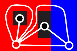
Figure 10: The primal graph correctly encoding the inclusion- and multiple border relationships between regions.

Damn! Still Not Enough Complex Graphs to Encode Images Properly???

I would say, that we already got to a point, where we can pretty well represent region layouts in an image using a small (dual) graph. But there is still one small problem – there may be some ambiguities. Let’s look at the figure below:

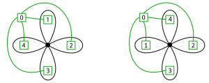
Figure 11: Ambiguities in the green primal and black dual graph.

Here we see two green primal graphs. Obviously, they have the same shape, but there is one small difference. The “1” and “4” regions are switched. And that is exactly the problem – both graphs look exactly the same! This way we can have two reduced image graphs, which look exactly the same but encode different region settings in the image.

To solve this problem, scientists came up with a different graph encoding, namely a combinatorial map. A graph is encoded as a set of vertices and edges. Contrary to this, a graph can also be encoded as a combinatorial map, which consists of a set of half-edges called darts, and two permutation functions:

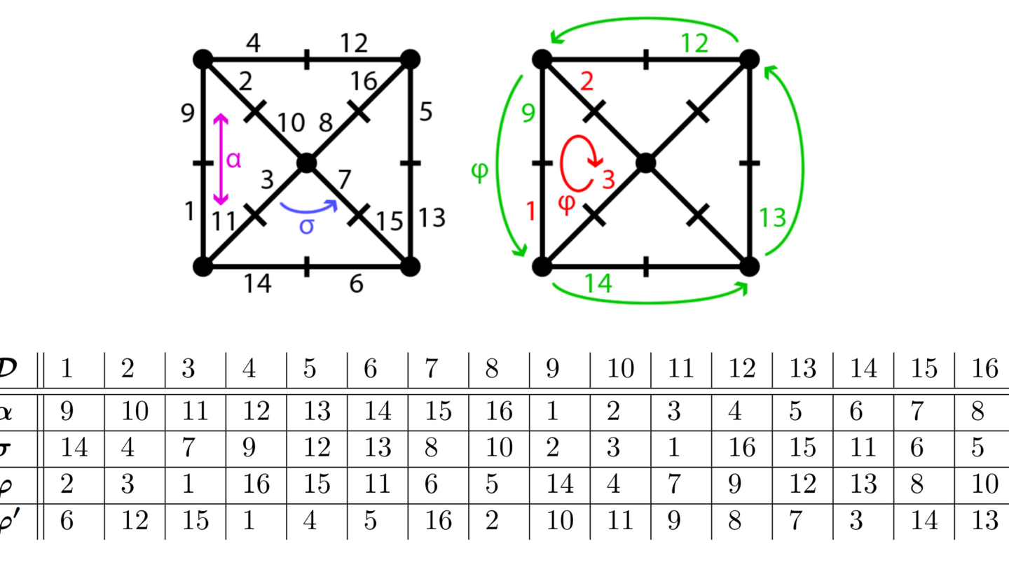
Figure 12: A combinatorial map consisting of 4 darts and 2 permutation functions α and σ.

In Figure 12 we see a very simple example of a combinatorial map. Here we have 4 darts, namely “1”, “2”, “3”, and “4”. And these darts are held together through 2 functions. The “alpha”-permutation always connects two darts, which build up together an edge. In this case the α-permutation would look like this: {(1,2), (2,1), (3,4), (4,3)}. And then there is the “sigma”-permutation, which connects two darts in the clockwise or counter clock-wise direction. This way the σ-permutation would look like this: {(1,1), (2,3), (3,2), (4,4)}. To give a little more complex example, look at the graph on the left side in the figure below.

Figure 13: A more complex combinatorial map.

The most interesting thing to notice here is, that a combinatorial map, which is just a different representation of a graph, implicitly contains the dual graph. What I mean by this is, that with only having the set of darts D, the alpha- and sigma- permutation, we can directly compute the dual combinatorial map from it. And this is very simply done by combining the two permutations into a new one, the “phi”-permutation, which connects two darts of edges, which build up the border of a face. The dual combinatorial map is shown in Figure 13 on the right side. I know, it may be a little bit complex by now, but I wanted to make a complete connection between dual graphs and dual combinatorial maps.

One last thing worth mentioning here is, that the dual graph reduction operations can very well be done in a combinatorial map scheme. Henceforth it is sufficient to change the sigma-permutation. In the vertex merging operation, we just connect the two darts around the new combined vertex. And the same applies to edge removal. In the sigma-permutation we just skip the darts, which build up the edge, that is removed. To simply illustrate it, look at the figures below:

Figure 14: A vertex merging operation, which changes the sigma-permutation into a new one.

Figure 15: An edge removal operation, which also only changes the sigma-permutation.

This way, a combinatorial pyramid is equivalent to a “normal” graph pyramid, which means that all of the properties of the “normal” graph pyramid also apply to the combinatorial one. The advantage however is, that we do not need to store two separate graphs (primal & dual), but it is sufficient to only store one (primal) combinatorial map. And now to end it all up, the main advantage is, that now we can uniquely encode a setting of regions! Look at the figure below:

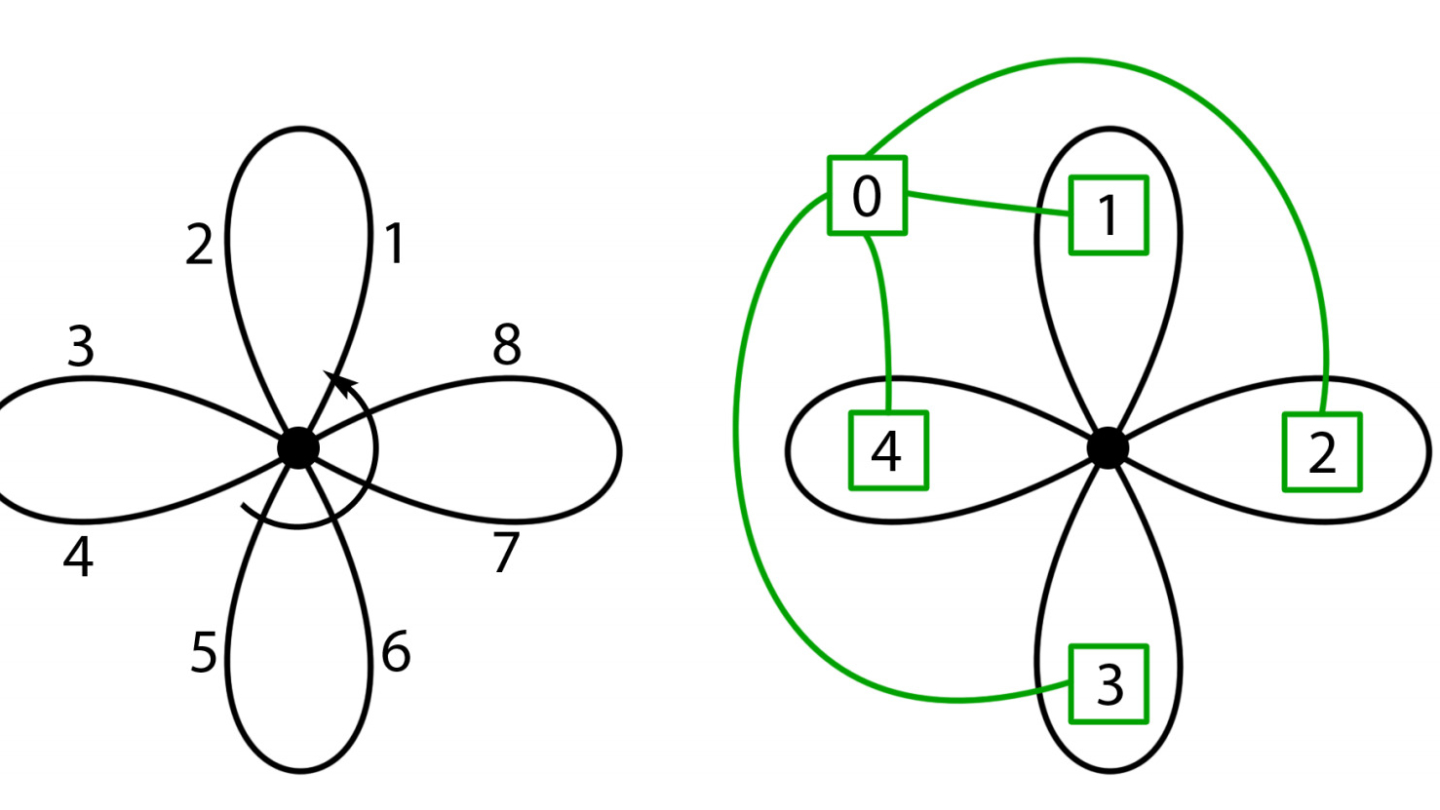
Figure 16: A combinatorial map and a dual graph.

With the dual graph representation, we were able to switch up vertices “1” and “4”, so that the two graphs would look exactly the same. With the combinatorial map encoding, this is however not possible anymore! When we would switch up the two vertices, then the dual combinatorial map shown in black on the left side of Figure 15 would change the sigma-permutation!

There is one more generalization of combinatorial maps, namely the generalized maps, but they are out of the scope of this blog post. Their advantage over the classical combinatorial maps is, that they can also represent non-orientable objects like the famous Möbius strip or the Klein bottle, depicted below.

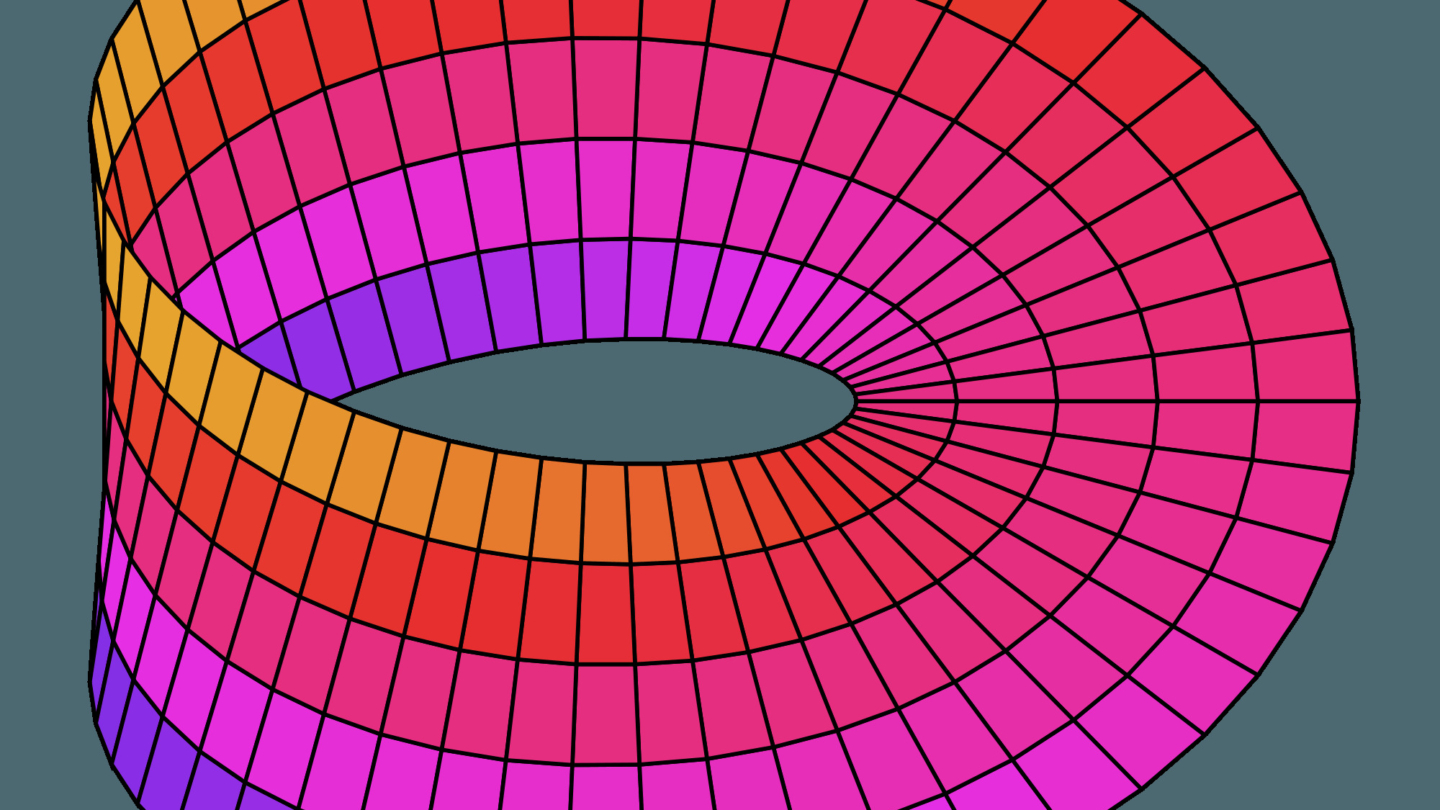
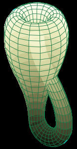
Figure 17: Non-orientable surfaces: Möbius strip on the left, and the Klein bottle on the right.

As you can see, each of the shown graph theoretical concepts has its own advantages and disadvantages. Some are simple but lack the ability to represent certain objects. Others are complex but can represent almost any surface. For this reason, before selecting a fitting graph concept, always look at what your requirements are and decide based on those.

Try our Demo App!