Introduction to Graph Theory – Part 1

In today’s blog post we will take a look at graphs – how and why they were invented, what they actually are, and what are their applications. Even though it is basically mathematics, and not so many people like mathematics 😀 , I will do my best not to go too deep into the mathematical part, and rather try to explain it on simple examples.

Graphs? What Do We Need Them For?

You may not be aware of it, but you get in touch with graphs on a day-to-day basis. You drive to work and use a navigation system to compute the time-optimal or shortest route? You use a computer and traverse the file system with an explorer application? You use Google to search for some specific keywords and you almost always get the best suggested results on the first page? Well, all of these tasks, and many many more, are accomplished by using graphs and their properties.

The first mentioning of a graph dates back to 1736, when the famous genius Leonhard Euler published his paper on the Seven Bridges of Königsberg. The setting was the following: the city of Königsberg was set on both sides of a river, and also included two islands. The two islands were connected to each other, and also to the both sides of the river (see image below). It may have been due to security- or sales reasons back then, but the problem was to find a walk, such that each bridge was crossed exactly once, and the starting point and endpoint did not have to be the same. This problem is nowadays also known as finding the existence of an Eulerian path, and back in 1736, Euler has shown that in the particular case of Königsberg, this problem could not be solved. With this paper, the basic graph theory was born.

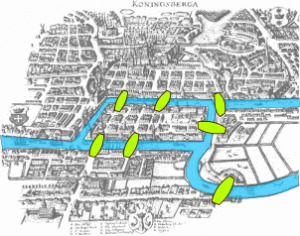
Figure 1: Königsberg and its seven bridges (source: Wikipedia).

Graph Definition and Some Real World Problems

The idea of Euler of how to solve the problem at hand was to model each side of the river and the two islands as points, and the bridges connecting these pieces of land as lines. In more mathematical terms, these points are called vertices, and the connecting lines are called edges. The simplest definition of a graph G is, therefore, G=(V,E), which means that the graph G is defined as a set of vertices V and edges E (see image below). With such a simple graph we can solve problems like the already mentioned Eulerian path problem, or its closely related Hamiltonian path problem, which requires a path to visit every single vertex of the graph.

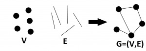
Figure 2: Construction of a simple graph.

With time more and more complicated graph problems arose, which required an extension of the simple graph definition. Among such extensions are the assignment of a weight w to an edge, an attribute a to a vertex, or even directions to the edges. Let’s think shortly about a map of a country. Here we could model the cities as vertices, the different roads connecting them as the edges, and the weights of the edges as the distances between the cities. We could also assign the population count of each city as an attribute to a vertex, and also in case of one-way streets a specific direction to the edges. When a road has no direction assigned to it, then it can be traversed in both directions.

In mathematical terms, an edge is expressed as a pair of vertices. For example, when a directed edge e connects the vertices v and u, while having the start point at v and endpoint at u, then it is written as e=(u,v). The same edge with the opposite direction would be mathematically expressed as e=(v,u). Finally, an undirected edge e can be expressed as e={u,v} or e={v,u}. Notice here, the only differences are the round and curly braces. An undirected edge essentially consists of two directed edges, which point in the opposite direction of each other:

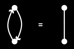
Figure 3: Undirected edges can be interpreted as two
directed edges pointing in the opposite direction.

Going back to the country map example – what advantage does it have to add all this additional information to a graph? Well, one of many problems which takes advantage is called the Traveling Salesman Problem. Imagine you are a traveling salesman, and you want to visit every single city with the least effort, that means traveling the least distance. This a very well studied optimization problem, that has its application in the real world. There are many many different approaches to solve this problem, globally optimal ones and approximative ones, but most of them work by subdividing the problem into smaller ones, and look for the locally optimal solution and then combine those into a globally optimal one. But that’s a topic for another time 😉

I Only See Trees in This Forest

Besides these intrinsic properties of the graphs like weights and directions, we also have different types of graphs, when it comes to their connectivity. There is for example the possibility, that two vertices are connected through multiple edges, called parallel edges. Another possibility is, that a vertex is connected to itself by an edge, which makes the edge a self-loop. Thinking at the map example, parallel edges would be multiple roads leading from one city to another one. Obviously, these edges can have different weights, when thinking about distances, because one road could be a direct highway, and another one could be a road, which leads around fields and forests. Following this analogy, then a self-loop would be a road, which would go out of town, around a forest, and then lead right back to the city (in case you would like forest sightseeing 😀 ). Anyway, there is a distinction between simple graphs, which may not contain any parallel edges and self-loop, and multi-graphs, which may have both of these characteristics.

Going at a little bit higher level, we may also look at whole paths (sequences of vertices and edges). If it is possible to follow a path, such that you start at a vertex, do not use an edge more than once, and come back to the starting vertex, then you have a cycle somewhere in your graph. On the other hand, if there is not a single cycle in your graph, and every vertex is connected to the same big connected component, then you have a so-called tree. This classification of a graph into a tree has also been made very early on, because of problems such as finding the Minimum Spanning Tree of a graph. Here the problem is the following: you have a weighted undirected graph, which possibly contains cycles. The main goal is to find a subset of edges, which connects all of the vertices in such a way, that there is no more cycle, and this set of edges has the minimal sum of the assigned weights. The first need for a solution to this problem was in 1926, when the Czech scientist Otakar Borůvka had to propose an efficient electrical covering of Moravia. The vertices here would correspond to the cities or electrical posts, and the edges the electrical connections. You surely can already see a pattern in this classification of graphs. With each completely new problem, a new classification of graphs is born 🙂

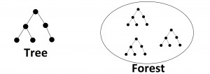
Figure 4: A forest is a collection of trees, and not only in graph theory 🙂

Analogously to the trees in a forest, you also have a forest of graphs, that are trees. Essentially you have a whole collection of vertices, that are connected in such a way, that there are more than two components, and none of these components contains a cycle. This ensemble of trees, is then called a forest in graph theory.

Finally, the last special type of graphs, that I would like to mention here are planar graphs. This type of graphs has the characteristic, that no two edges of the graph can cross each other. Planar graphs are very often used in Computer Vision to represent images. You have the individual pixels, which are represented as vertices, and then you have the edges, which connect the top, bottom, left, and right neighboring pixels. Such image graphs usually have stored the pixel color values stored as attributes at the vertices, and the color differences as weights at the edges. One of the most commonly solved problem in Computer Vision using image graphs is Image Segmentation. Here, the problem is to divide the image into groups of pixels in such a way, that the pixels which belong to the same region share some common properties, such as similar color or texture, and the pixels belonging to two different regions are dissimilar with respect to these properties. An example of a result of an image segmentation can be seen in the image below.

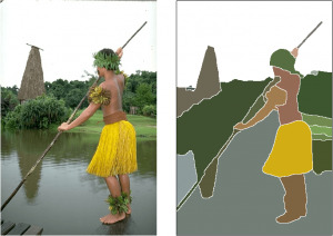
Figure 5: An example image on the left is segmented to regions with similar color.

As you can see, with each new problem a new classification and extension of graphs were necessary. Currently, there are thousands of problems that can be solved with graphs (even a deep neural network representation problem ). Let’s see what new graph-related problems will occur in the future, and even more interesting, what solutions will be proposed 🙂

In the next part of our introduction to graph theory, we will take a look at more complex, hierarchical graph concepts, which are quite often used in Computer Vision for tasks such as image segmentation, structural pattern recognition, etc.

Try our Demo App